

Guide to Transformer Loss Data Analytics
A transformer can be more than 99% efficient and still waste tens of thousands of dollars per year. I’d break this topic down into four parts: what losses are, which data to track, how to clean that data, and how to use it for maintenance and buying decisions.
If I wanted the short version, it’s this:
- No-load loss runs all the time, even at light load.
- Load loss climbs with current and heat, and it grows fast at high load.
- Hot-spot temperature helps estimate insulation aging and loss-of-life.
- Power quality issues like harmonics and unbalance can add extra loss.
- Bad meter accuracy or poor timestamp alignment can hide the loss signal.
- Cost models turn kW loss into annual dollars and long-term ownership cost.
- Advanced models help when heat, harmonics, and unbalance hit at the same time.
A few numbers make the point fast:
- A 20,000 kVA transformer at $0.10/kWh can lose about $38,690 per year in energy.
- A 1,000 kVA unit may have 1.0–1.5 kW of no-load loss and 12–16 kW of full-load loss.
- Winding resistance rises about 0.4% per 1°C increase in temperature.
- Monitoring can give 30 to 120 days of warning before failure.
- One cooling issue fixed in the field cut winding temperature by 20–40°C (68–104°F).
If I were setting up a loss analytics program, I’d start with the factory test report, add current, voltage, power factor, temperature, DGA, and harmonic data, then normalize the readings before trending them. From there, I’d use the results to spot drift, estimate aging, rank fleet risk, and compare new versus used transformer options by total cost over service life, not just purchase price.
That’s the whole article in plain English: measure the right signals, clean the data first, then use the output to cut waste, lower failure risk, and make better buy/replace calls.
Electrical Transformers Efficiency Analysis Dashboard - Part 1 - Power BI
sbb-itb-501186b
Transformer Loss Fundamentals and the Data You Need
Once you know what those losses cost, the next job is simpler in theory and messier in practice: figure out which loss types your data can separate.
Main Loss Categories and How They Show Up in the Field
Transformer losses fall into four main types, and each one leaves a different fingerprint in the data.
No-load losses stay almost flat any time the transformer is energized. Load losses climb with current and temperature.
Stray losses come from leakage flux in metal parts, and they increase when the transformer feeds harmonic-heavy, nonlinear loads. If those nonlinear loads are also unbalanced, 3rd- and 5th-harmonic losses go up as well.
Dielectric losses happen in the oil and paper insulation. In most cases, they matter mainly on units above 100 kV.
Tests, Standards, and Reported Values
Open-circuit and short-circuit tests set the no-load and load-loss baselines that analytics models use.
The main standards here are:
- IEEE C57.12.90 for liquid-immersed transformers
- IEEE C57.110 for harmonic losses
- ANSI/UL 1561/1562 for dry-type units
IEEE standards permit a manufacturing tolerance of ±10% on load losses and ±15% on no-load losses.
When you compare load losses, make sure they're normalized to a reference temperature first. That's usually 75°C or 85°C for oil-immersed units and 105°C for dry-type units. If you skip that step, you're not making a clean apples-to-apples comparison.
Key Inputs for Analytics Models
A useful model needs three inputs at a high level: a factory baseline, live operating data, and economic context.
| Data Category | Key Variables | Use in Analytics |
|---|---|---|
| Nameplate | Rated kVA and cooling class, voltage, impedance, X/R ratio | Establishes baseline capacity and efficiency curves |
| Factory Test | No-load loss, load loss at reference temperature | Provides the constants for the loss formula |
| Operating | Current, voltage, power factor, tap position | Calculates real-time load percentage and power flow |
| Thermal | Winding temp, top-oil temp, ambient temp | Corrects resistance-based losses for actual heat levels |
| Power Quality | THD, 3rd/5th harmonic levels | Identifies additional losses from nonlinear loads |
| Economic | Energy rate ($/kWh), annual hours, load factor | Converts physical energy loss into financial cost |
Use the factory test report as your baseline. For field verification, calibrated Rogowski coils are a strong fit because they stay linear and can reach 0.01% accuracy or better.
These inputs set the baseline. The next section turns that baseline into a live monitoring pipeline.
How to Build a Transformer Loss Monitoring Data Pipeline
With baseline inputs defined, the next job is getting solid field data into the analytics stack.
Sensors, Meters, and Online vs. Offline Measurements
Transformer losses are only 0.5–2% of rated power, so even small meter error can hide the loss signal. That means accuracy matters a lot. Use high-accuracy current, voltage, and power meters, because minor phase or ratio errors can throw off loss calculations fast. Once the baseline is set, the focus shifts to gathering field data without losing that signal in the noise.
You also need more than electrical readings alone. Add thermal, gas, moisture, and bushing sensors to get a broader condition view. Here’s what each parameter is tracking:
| Parameter | What It Monitors |
|---|---|
| Oil Temperature | Overloading, cooling failure |
| Winding Hot Spot | Insulation breakdown risk |
| Dissolved Gas (DGA) | Arcing, partial discharge |
| Moisture Content | Insulation degradation |
| Load Current | Overload trends |
A simple way to think about it: factory test reports give you the starting line, and live sensors show how far the transformer drifts from it over time.
Data Acquisition, Communications, and System Integration
DAUs or IEDs digitize the signals, and edge processing can send trends instead of raw streams. From there, data flows into SCADA or Energy Management Systems (EMS) through Modbus, DNP3, or IEC 61850 protocols.
In high-voltage substation settings, optical fiber transceivers and multiprotocol converters help protect communications from electromagnetic interference (EMI). After collection, the data lands in local historians, asset management platforms, or cloud analytics environments. That’s where cross-facility benchmarking and digital twin modeling start to make sense.
If billing and metering points don’t match, loss-compensation meters can calculate losses automatically. Get the acquisition layer right, and your trending, aging analysis, and fault detection have a much better shot at being accurate.
Data Quality Checks Before Analysis
Bad data leads to bad calls. Before analysis starts, three checks matter most.
- Timestamp alignment: Electrical variables may sample every 30 seconds, while DGA and temperature channels often update every 1 to 5 minutes. If you combine those streams without lining up timestamps, you can create false correlations. GPS-based phase synchronization is critical for accurate phase angle measurements across distributed sensors.
- Temperature correction: Normalize load-loss data to a reference temperature before trending.
- Outlier detection: Trending algorithms should flag unrealistic readings as possible sensor faults, not asset faults. For DGA, start trend analysis above 50 ppm to avoid false positives from baseline noise.
One more practical step: keep raw, normalized, and log tables separate to preserve lineage and auditability.
With aligned and normalized data in place, analytics can move from simple measurement into loss tracking, aging analysis, and risk detection.
Analytics Methods for Monitoring Losses, Aging, and Fault Risk
Once the data is clean, the job shifts from collecting readings to turning those readings into signals you can act on: cost, aging, and fault risk.
Rule-Based Calculations, Trending, and Cost Tracking
A good place to start is the efficiency ratio:
η = P_out / (P_out + P_core + P_cu)
Track it over time to spot drift away from the design point. Peak efficiency happens where core loss and copper loss are in balance, though the exact load point varies by transformer design. The point isn't just to estimate loss. It's to figure out where action matters most.
Start simple. Rule-based methods are often enough at first. If harmonics, phase unbalance, or temperature begin to muddy the signal, then it makes sense to step up to more advanced models.
You can also turn efficiency trends into direct cost impact with:
Annual Cost = (P_NL × 8,760 + P_LL × LF² × operating hours) × $/kWh
| Approach | Required Inputs | Complexity | Strengths | Limits |
|---|---|---|---|---|
| Rule-Based Thresholds | Nameplate data, OEM test reports, basic SCADA | Low | Fast to deploy; works well under standard conditions | Misses harmonics, unbalance, and other composite effects |
| Trend Analysis | Time-series load and temperature data | Low–Medium | Useful for spotting gradual drift | Can miss short, event-driven issues |
| Basic Cost Estimation | Load factor, energy rate, loss values | Low | Turns losses into dollar figures | Assumes a stable load profile |
| PCA-reduced neural model | Multi-source electrical data reduced with PCA | Medium | Helpful for unbalanced loads and low-voltage recovery | Still depends on high-quality historical data |
| Transformer-BiLSTM hybrid | High-resolution power-quality data | High | High precision (<0.18% error); captures multi-factor coupling | Requires strong preprocessing and validation |
That table tells a pretty simple story: low-effort methods are good for day-to-day monitoring, but they start to struggle when multiple disturbances hit at once.
Thermal Aging, Loss-of-Life, and Condition-Specific Analysis
Temperature normalization helps separate actual aging from plain resistance drift. For oil-immersed units, the normal reference is 75°C or 85°C. That matters because transformer aging isn't driven by one number alone. Hot-spot temperature, top-oil temperature, ambient conditions, and loading level all work together to shape the real loss-of-life under field conditions.
Ambient heat can push losses up fast. When temperatures go above 104°F (40°C), losses can run 15% to 20% above nameplate values. In summer, that isn't just a spreadsheet issue. It can turn into an operating limit.
Voltage deviation has the biggest effect on losses, with three-phase unbalance next, followed by third harmonics. In distribution systems, neutral line current is worth tracking too. That's because three-phase unbalance increases zero-sequence losses, and standard balanced-load models can miss them.
Machine Learning and Advanced Validation
Advanced models start to earn their keep when transformers face composite disturbances - harmonics, voltage deviation, and load unbalance at the same time. That's where rule-based methods tend to lose their grip.
Hybrid deep learning setups such as the Transformer-BiLSTM hybrid use a Transformer encoder to pull out global features, then BiLSTM layers to track temporal behavior. In field comparisons, this approach reached loss prediction error below 0.18% and similarity coefficients above 0.9989 against actual measurements.
That level of accuracy matters even more when you compare it with instrumentation limits. Standard Class 0.5 current and voltage transformers bring 1–2% measurement error, which is often larger than the losses being measured.
A practical rule is simple: move past rule-based analysis when composite disturbances show up often, or when the loss signal gets close to measurement noise. Before trusting the output, validate it against at least 7 days of consecutive field data and benchmark it against BP, GA-BP, and PSO-BP results. Once the model is checked, its output can be used to rank assets and support transformer selection and deployment.
Applying Analytics to Transformer Selection, Deployment, and Long-Term Decisions
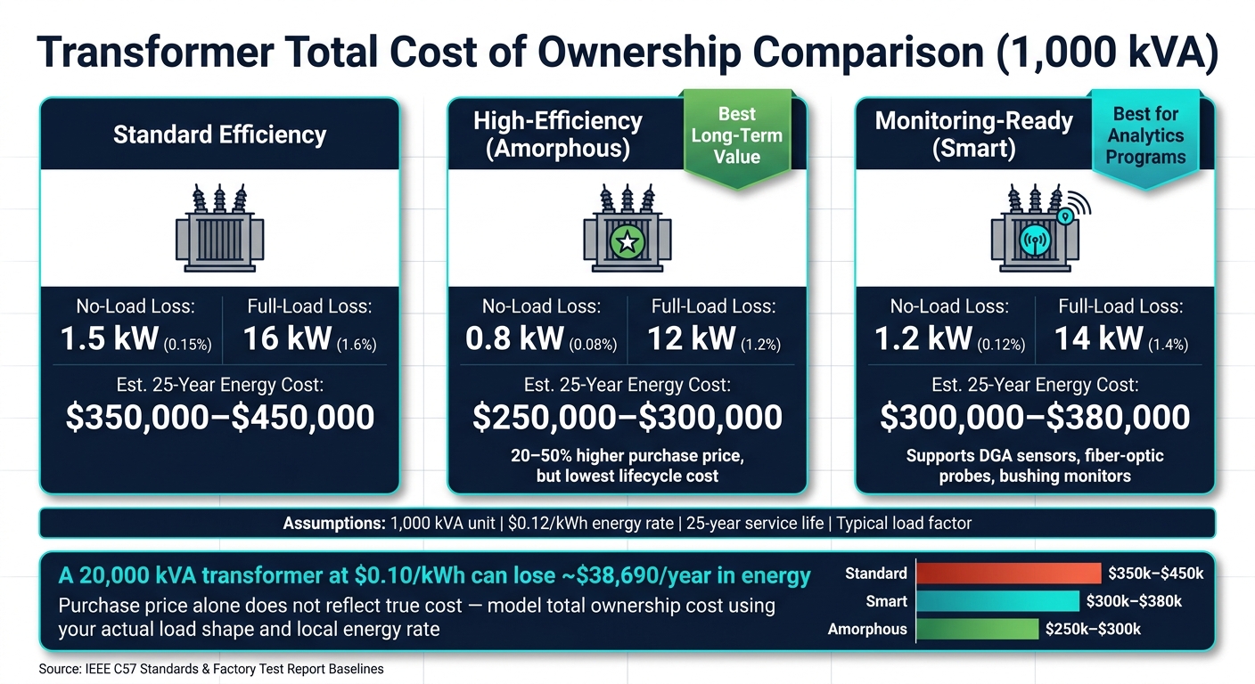
Transformer Total Cost of Ownership: Standard vs. High-Efficiency vs. Smart Units
Using Loss Analytics to Choose the Right Transformer
Once your trending and aging models put numbers on operating loss, you can use that same data to compare transformer options before you buy. And that matters, because the sticker price doesn't tell the whole story.
A lower-cost unit can end up costing more over a 25- to 40-year service life once no-load and load losses are included. The smarter move is to run the same loss model across each candidate transformer and compare total ownership cost, not just purchase cost. This is especially important when the transformer will spend much of its time below full load, since partial-load operation can shift lifecycle cost in a big way.
Representative 25-year energy-cost estimates at $0.12/kWh are shown below:
| Transformer Type (1,000 kVA) | Typical No-Load Loss | Typical Full-Load Loss | Est. 25-Year Energy Cost ($0.12/kWh) |
|---|---|---|---|
| Standard Efficiency | 1.5 kW (0.15%) | 16 kW (1.6%) | ~$350,000–$450,000 |
| High-Efficiency (Amorphous) | 0.8 kW (0.08%) | 12 kW (1.2%) | ~$250,000–$300,000 |
| Monitoring-Ready (Smart) | 1.2 kW (0.12%) | 14 kW (1.4%) | ~$300,000–$380,000 |
High-efficiency units often come with a 20–50% price premium, but analytics can show where the break-even point lands by modeling your actual load shape and local energy rate. Also, don't rely on brochure numbers alone. Check the baseline no-load and load-loss values in the factory test report.
Sourcing Monitoring-Ready Equipment and Planning Installation
The cost model should feed straight into your purchase spec. If monitoring matters, put it in the purchase order from the start instead of treating it like an add-on later.
A unit that already supports dissolved gas analysis (DGA) sensors, fiber-optic temperature probes, and bushing monitors gives your analytics pipeline clean input from day one. That makes setup easier and helps avoid patchwork retrofits later.
Metering accuracy also needs to be tighter than the loss signal you're trying to detect. If the meter can't see the change, the model can't help you much.
The same loss data used for selection can also help with refurbish-versus-replace calls. On tighter budgets, reconditioned transformers can often be sourced at 30–60% of new-unit pricing, while refurbished units with warranties usually land at 50–75% of new cost. Before buying any used unit, review its full DGA history and loading records, since those records feed straight into loss and aging models.
Electrical Trader lists new and used transformers along with supporting equipment, which makes it a practical place to compare specs and maintenance history against lifecycle cost targets.
Conclusion: Key Decisions That Improve Efficiency and Reliability
Turning raw sensor data into better capital decisions usually comes down to a few basic moves: know which loss mechanisms apply to your equipment and load profile, build a data pipeline with sensors that can detect the signals that matter, and check data quality before trusting the output.
From there, those results can guide transformer selection, installation planning, and replacement priority across a fleet. But the output is only as good as the data and models behind it.
"The value of a transformer monitoring is not determined by how much data it collects, but by how effectively that data improves decision-making." - Rugged Monitoring
FAQs
How do I start tracking transformer losses?
Start with the manufacturer’s factory test report. That report gives you the baseline for load losses and no-load losses.
For day-to-day monitoring, collect steady-state voltage and current readings at the transformer’s low-voltage terminals. If you want direct field measurements, use high-precision power analyzers and instruments with at least 0.5 class accuracy.
Here’s why that matters: standard power metering often isn’t precise enough to measure these small losses well.
What data quality issues matter most?
The biggest trouble spots are meter accuracy and calibration, data interval length, and power quality.
Commercial meters can add 1%–2% error. In some cases, that’s more than the losses you’re trying to measure in the first place.
Data resolution matters just as much. Lower-resolution readings, like 15-minute or 30-minute intervals, can understate losses by up to 40% compared with 1-second data.
Power quality can throw things off too. Voltage deviation, phase unbalance, and harmonics can all increase losses and distort the math if you don’t correct for them.
When should I use advanced loss models?
Use advanced loss models and direct measurement when standard manufacturer data or rule-of-thumb estimates fall short.
They matter most in high-frequency work, especially with ferrite cores or iron powder materials, where losses change with frequency and need precise, real-time analysis.
They also play a big role when power quality gets messy, like with high harmonic distortion or unbalanced loads. The same goes for research, compliance testing, or any decision that calls for sub-0.1% measurement accuracy.