Predictive Analytics for Load Forecasting

July 13, 2026

If you want better load forecasts, I’d keep it simple: use clean load and weather data, match the model to the forecast window, and only use the forecast when it leads to a clear action.

In this article, I walk through the full path from meter data to decision-making. The core idea is straightforward: bad inputs lead to bad forecasts. So I start with AMI, SCADA, feeder, PDU, and weather data, clean gaps and spikes, convert three-phase readings into active power (kW), and build time, weather, and event features. From there, I pick a model based on the job: SARIMA for steady seasonal patterns, Random Forest or XGBoost for weather-driven load shifts, and LSTM for dense 15-minute interval histories.

Here’s the article in one quick list:

I explain which forecast horizon fits which decision, from 1–30 minutes up to multi-year planning.
I show which data sources fit each target, including AMI, SCADA, feeder meters, PDU data, and weather feeds.
I cover data cleaning, including gap filling, outlier checks, timestamp alignment, and weather resampling.
I include the three-phase power formula: P (kW) = (√3 × V<sub>L-L</sub> × I × PF) ÷ 1,000.
I compare model types based on seasonality, nonlinear load behavior, compute needs, and explainability.
I validate forecasts with MAE, RMSE, and MAPE, with extra focus on RMSE when peak misses matter most.
I use walk-forward validation instead of random splits to avoid leakage from future data.
I connect forecast output to actions like dispatch, switching, maintenance timing, load transfer, and equipment buying.

A few facts stand out. The article notes that by the end of 2018, U.S. smart meter deployments reached about 86 million. It also points out that even small accuracy gains in short-term forecasting can cut operating cost by improving dispatch choices. And for systems with DERs and EV charging, higher-frequency data like 5-minute or 15-minute intervals helps show load patterns that older methods can miss.

If I had to boil the whole piece down to one line, it would be this: forecast only what you can use, measure the error honestly, and tie every forecast to a threshold that triggers a decision.

Forecast Electricity Demand With Predictive Analytics And Alteryx | Continuum

Alteryx

Step 1: Prepare Load and Weather Data

Start by matching the data source to the forecast horizon. AMI works well for building-level, short-term forecasts. SCADA and feeder meters fit circuit-level forecasting. PDU meters are used for plant loads. And weather data matters when demand shifts with temperature.

Short-term forecasting needs inputs that match the same interval. Long-term planning usually calls for cleaner aggregated data with fewer gaps. From there, align every source to the same interval, unit, and forecast target.

Choose Data Sources Based on Your Forecasting Goal

Data Source	Coverage Level	Time Resolution	Common Use Cases	Limitations
AMI (Smart Meters)	Individual building	15 to 60 minutes	Demand response, billing, behavior analysis	High data volume; privacy concerns
SCADA / Substation	Substation / feeder	Seconds to minutes	Grid stability, outage management	Aggregated view; less detail at the customer level
Feeder Meters	Feeder / neighborhood	1 to 15 minutes	Localized load balancing, phase balancing	May miss individual building fluctuations
PDU / Facility Metering	Equipment / floor	1 to 15 minutes	Plant scheduling, equipment maintenance, peak shaving	Limited to specific industrial sites
Weather APIs	Regional / local	Hourly to daily	Input feature for all forecasting horizons	Accuracy depends on station proximity

For short-term load forecasting, begin with 15-minute to hourly AMI, SCADA, and feeder data. Align all of it to the same local timestamp as the weather source. If one stream is off by even a little, the model can end up learning the wrong pattern.

Clean, Validate, and Build Forecast Features

Raw AMI and SCADA data often comes with gaps, spikes, or timestamp mismatches. Clean that up before training.

Use linear interpolation for short gaps. For longer outages, replace missing values with same-day, same-season historical averages. Remove or flag outliers caused by bad meter reads. Then resample weather data to the forecast interval before merging it with load data. That step sounds small, but it can make or break the input set.

Once the data is cleaned, build features that help the model spot patterns:

Calendar features: hour of day, day of week, month, season, and U.S. holiday flags
Weather variables: temperature in °F, relative humidity, heat index, and, when available, solar radiation, wind speed, and precipitation
Event flags: planned outages, maintenance, and atypical plant schedules

This is where the forecast starts to feel grounded in how the site actually runs, not just what the meter happened to record.

Calculate Three-Phase Load Inputs Correctly

The model input should be active power in kW, not raw current or voltage readings. For a balanced three-phase system, use this formula:

P (kW) = (√3 × V_L-L × I × PF) ÷ 1,000

Where V_L-L is the line-to-line voltage in volts, I is the current in amps, and PF is the power factor.

Before you aggregate three-phase measurements into the model, verify that the phases are balanced. If they aren't, active power gets distorted, and that bias carries straight into the forecast.

With clean inputs expressed as active power, the next move is picking the model that matches the load pattern.

Step 2: Select and Build a Forecasting Model

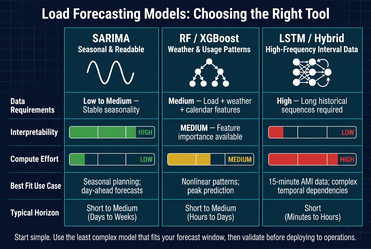
Load Forecasting Models Compared: SARIMA vs. Random Forest vs. LSTM

Once your active-power inputs are ready, pick a model that fits the forecast horizon, the amount of data you have, and how much explanation the forecast needs.

That choice comes down to a practical question: What is this forecast being used for? A model for feeder overload decisions may not be the same one you'd use for transformer risk checks or dispatch planning. In most cases, it's smart to start simple. Use the least complex model that fits the forecast window, then validate it before putting it into operations.

Use SARIMA for Seasonal and Readable Forecasts

SARIMA works well for stable feeder or substation loads with clear seasonality. It's efficient to run, and its forecasts are easy for engineers and planners to read and explain.

Start by testing for stationarity. If the series isn't stable, difference it until the mean and variance settle down. Then fit the model for the forecast horizon you need, like day-ahead or week-ahead forecasting.

SARIMA is a good baseline for stable feeders with regular seasonal patterns.

Use Random Forest or XGBoost for Load Patterns Driven by Weather and Usage Interactions

Sometimes load doesn't move in a simple straight-line way. Temperature in °F, humidity, and time of day can interact in messy ways, and that's where tree-based models come in handy.

Random Forest and XGBoost can learn from lagged load values, calendar features, and weather variables without assuming linear relationships. That makes them useful when load shifts with weather and usage behavior at the same time.

Another plus: feature importance gives operators a clearer view of what's driving load. For example, it can help flag weather-driven peak risk on feeders or transformers.

Use LSTM or Hybrid Models for 15-Minute Interval Data

For 15-minute AMI or facility-meter data, especially when you have long histories and changing consumption patterns, LSTM networks are often a strong match.

They are built to hold patterns across long sequences, which helps with complex time-based dependencies. In plain terms, they can track how earlier behavior affects later load in ways simpler models may miss.

LSTM fits long, high-frequency load histories well, but there are tradeoffs. It needs more compute, and it is harder to explain to operations teams.

The table below shows where each model type tends to fit across the main decision factors:

Model Type	Data Requirements	Interpretability	Compute Effort	Best Fit
SARIMA	Low to medium; stable seasonality	High	Low	Seasonal planning; day-ahead forecasts
RF / XGBoost	Medium; load + weather + calendar	Medium (feature importance)	Medium	Nonlinear patterns; peak prediction
LSTM / Hybrid	High; long historical sequences	Low	High	15-minute AMI data; complex temporal dependencies

Next, test the model with rolling validation and error metrics before using it in operations.

Step 3: Validate Accuracy and Apply Forecasts to Operations

A model can look solid in a report and still fall apart once crews start using it. Before you use any forecast to make actual distribution calls, test it the same way it will be used on the job.

Measure Forecast Error With the Right Metrics

After you pick a model, validation tells you if it’s fit for operations.

Use MAE to measure the average miss, RMSE when you care more about large misses and peak risk, and MAPE to compare feeders or substations with different load sizes.

Each metric tells you something different. If you under-forecast, overload risk goes up. If you over-forecast, operating cost goes up. That’s why RMSE often gets the nod when the main goal is to avoid overloads and big misses.

Use Walk-Forward Validation and Scenario Forecasts

A standard train/test split sounds fine at first, but it doesn’t hold up well for load data. If you split the dataset at random, future data can slip into training. That makes accuracy look better than it is.

The better option is walk-forward validation. You train on past data, test the next interval, then move the window forward. That lines up with how forecasts work in operations, where you only have past data when it’s time to make a call.

Scenario forecasts help too. Test normal conditions, hot-weather cases, and high-demand cases. That gives planners a practical demand range to use for reserve planning.

Validation Method	Robustness	Complexity	Fit for Operations
Simple Train/Test Split	Low; ignores temporal shifts and risks leakage	Low	Poor; does not reflect real-time updates
Walk-Forward (Rolling)	High; mirrors real-world data arrival and prevents leakage	Medium	Excellent; simulates daily/hourly dispatch cycles
Scenario-based	Very High; quantifies risk and uncertainty for peak demand	High	Critical for reserve planning and risk management

Turn Forecast Results Into Dispatch and Planning Actions

Once the model clears validation, plug the output into operating thresholds.

Match each forecast to a single decision, such as real-time dispatch, day-ahead switching, maintenance scheduling, or capital planning. For facility managers and contractors, forecast output can also shape equipment buying timelines. If the forecast points to steady load growth over the next year or longer, that’s a sign to start planning for new transformers or other equipment before capacity gets tight.

Set the decision threshold first. Then use the forecast only where its error stays below that limit. Those thresholds shape the equipment and risk calls that come next.

Conclusion: Use Forecasts to Plan Equipment and Cut Risk

After model validation, the forecast should become an operating trigger, not just an analytic result. Load forecasting only matters when it leads to a decision. Start with clean data, pick the right model, and validate it before you use the output to act.

From there, the forecast should guide equipment timing. Medium-term forecasts can help teams schedule maintenance and outage work before peak periods hit. If a forecast shows a feeder getting close to its thermal limit during peak periods, that should trigger upgrade or procurement planning.

When procurement lines up with projected load growth, teams can avoid the scramble of sourcing critical equipment under pressure. Forecasts can also help teams buy transformers, breakers, and other parts before capacity constraints become urgent.

The goal is simple: match the model to the forecast horizon, validate it honestly, and connect each forecast to a clear operating or procurement threshold. Use the forecast when it maps directly to an action, such as load transfer, maintenance timing, or equipment replacement.

Key Takeaways for U.S. Electrical and Facility Teams

The best forecast is the one that fits your data, time horizon, and decision. Match the method to the job, validate it honestly, and tie each forecast output to a threshold that triggers a real action.

FAQs

How much historical data do I need?

It depends on the model you use and how much you group the data.

Statistical methods like ARIMA can work well when you have historical time-series data. But there’s a catch: they still rely on high-quality data. If the input is messy, the output usually is too.

LSTM models, on the other hand, need larger datasets and more computing power. They can be a good choice when you have enough data and the setup to support them.

For simpler or smaller datasets, SVR is often a better fit. It’s easier to work with in those cases and can still deliver high accuracy.

What forecast horizon should I start with?

Start with the time horizon that fits your operational goal.

Use 5 to 60 minutes for automatic generation control, frequency regulation, or anomaly detection. Use a few hours to 1 day for energy transaction planning, unit commitment, or day-ahead dispatch. Use several months to over 1 year for capacity planning or infrastructure development.

Your data setup also needs to match that window. Shorter, high-frequency intervals often need more computing power, so it’s smart to check that your systems can handle the load before you commit to that range.

How do I know if my forecast is accurate enough to use?

Check your load forecast against operating targets and error metrics. For 1-hour forecasts, a common benchmark is MAPE below 2%.

That said, accuracy isn't the only thing that matters. Your control systems also need to respond fast, with latency under 100 milliseconds, so the grid can react in time instead of lagging behind events on the ground.

Operators often look at nRMSE and nMBE too. And in some cases, models have reached nRMSE as low as 2.76%.