

7 Metrics for Predictive Maintenance ROI
If you want to prove predictive maintenance ROI, I’d start with seven numbers before I buy anything: downtime hours, repair spend, asset life, alarm accuracy, labor hours, spare parts use, and outage frequency.
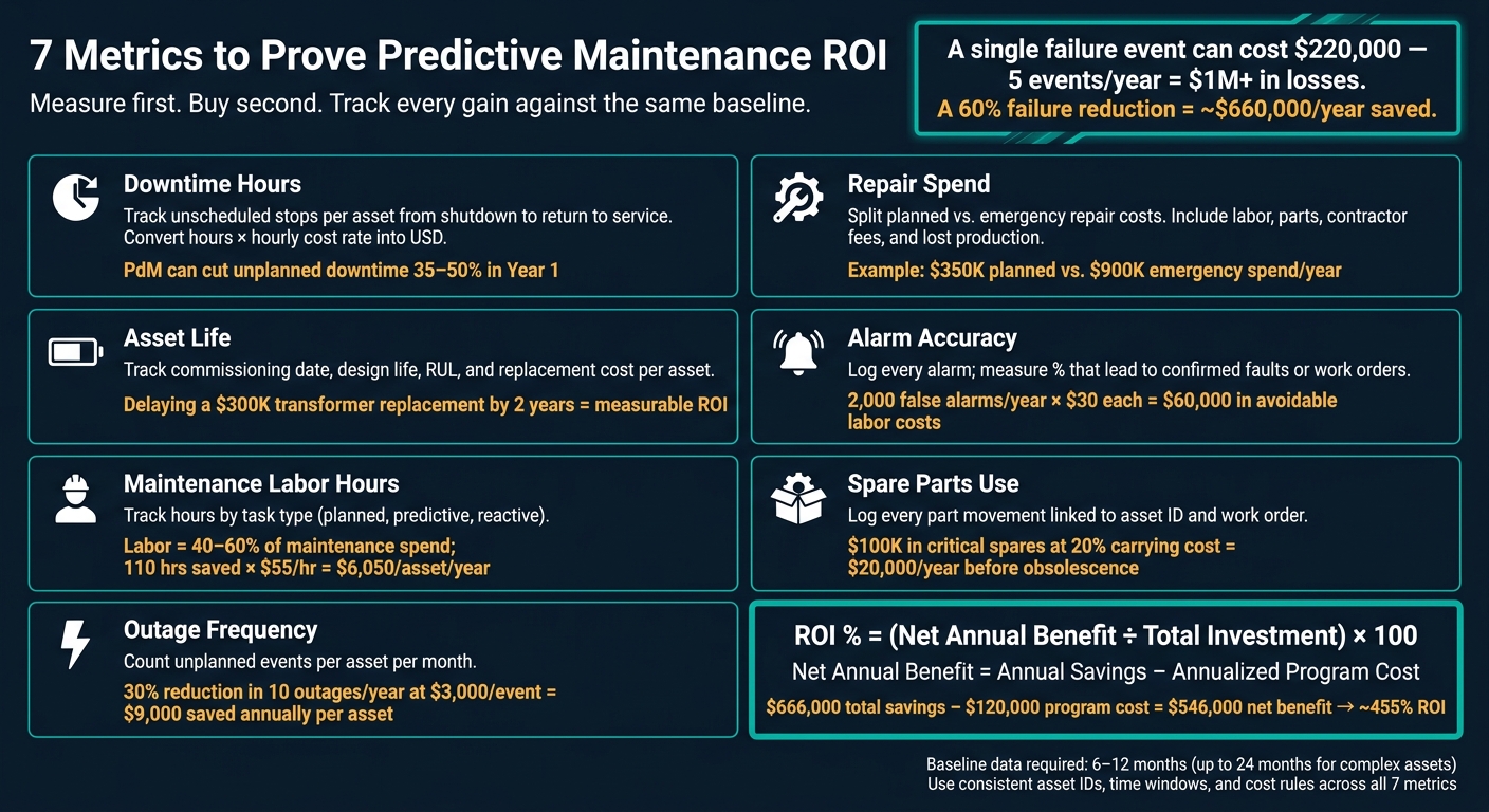
The article’s core point is simple: measure first, buy second. A plant can lose $220,000 per failure event, and five events a year can push losses past $1 million. If failures drop by 60%, that can mean about $660,000 per year back. But I can’t show savings like that without a baseline.
Here’s the short version of what matters most:
- I need 6–12 months of baseline data, and sometimes up to 24 months
- I should pull data from systems I may already have, like CMMS, SCADA, outage logs, labor records, and inventory records
- Each metric needs the same asset IDs, time windows, and cost rules
- I should convert each metric into U.S. dollar impact per year
- I need to avoid counting the same savings twice
A simple ROI model looks like this:
ROI % = (Net Annual Benefit ÷ Total Investment) × 100
And:
Net Annual Benefit = Annual Savings - Annualized Program Cost
The seven metrics covered in the article are:
- Downtime Hours
- Repair Spend
- Asset Life
- Alarm Accuracy
- Maintenance Labor Hours
- Spare Parts Use
- Outage Frequency
7 Predictive Maintenance Metrics: ROI Baseline Tracker
AI in Manufacturing: Predictive Maintenance for ROI & Uptime
sbb-itb-501186b
Quick Comparison
| Metric | What I’m measuring | Why it matters in dollars |
|---|---|---|
| Downtime Hours | How long assets are down | Lost output, restart cost, repair cost |
| Repair Spend | Planned vs. emergency repair cost | Shows where breakdowns drain budget |
| Asset Life | Age, remaining life, replacement timing | Helps price repair vs. replacement |
| Alarm Accuracy | How many alarms lead to action | Cuts wasted labor and alarm noise |
| Maintenance Labor Hours | Time spent by task type | Shows labor cost tied to failures |
| Spare Parts Use | Parts issued by asset and event | Tracks stock cost and rush orders |
| Outage Frequency | How often assets fail | Shows repeat failure patterns |
The bottom line: this article is about building a clean before-and-after scorecard so I can test vendor claims against my own plant data and put ROI in plain numbers.
Why These 7 Metrics Matter Before You Buy
Vendor ROI claims are based on averages. That sounds fine on paper, but your plant needs a baseline built from its own data. That’s what turns a rough estimate into an ROI case people can trust.
Each of these seven metrics ties back to a measurable cost or reliability loss: downtime, repair spend, asset life, alarm trust, labor, spare parts, and outages. Without that baseline, any promised gain is still just theoretical.
Just as important, baseline data gets operations, maintenance, finance, and reliability working from the same set of numbers. That cuts down on guesswork and helps teams talk about the business case in plain terms.
These seven metrics are the minimum dataset for a defensible ROI model. Start with downtime hours, then track the other six the same way.
1. Downtime Hours
Unplanned downtime hours give you a baseline for what equipment failures are costing. Track those hours for each critical asset, then turn them into dollars.
Start by defining what counts. Treat unplanned downtime as any unscheduled stop caused by asset failure, from shutdown to return to service. For example, if a generator trips offline, that full outage window counts.
Log every event in your CMMS or EAM system using the same fields each time:
- asset ID
- start time
- end time
- total duration in hours
- root cause code, such as mechanical, electrical, or controls
That consistency matters. If your fields shift during the baseline period, your numbers get messy fast.
Once you have the hours, convert them into dollars. Multiply downtime hours by the hourly cost for each asset. That cost should reflect lost output, labor, restart costs, and scrap. If a line makes 1,000 units per hour at a $2 margin per unit, it loses about $2,000 per hour before overtime and emergency repair costs. Assign a USD hourly cost to each asset and keep it the same through the full baseline period.
Then track repair spend using the same asset IDs and event records. That asset-level setup - unique IDs, fixed definitions, and a cost-per-hour figure - is what lets you compare before and after without guesswork.
Industry data suggests predictive maintenance can cut unplanned downtime by 35% to 50% in year one compared to reactive maintenance. Use that same tracking structure when you measure repair spend.
2. Repair Spend
Track repair spend for each critical asset with the same asset IDs and time stamps you use in your downtime logs. That shared structure is what links repair cost to each failure event. In your CMMS, log:
- asset ID
- date and time
- work type
- labor hours
- labor cost
- parts cost
- contractor fees
- total repair cost
Use a required Work Type field with options such as "Planned – Preventive", "Planned – Predictive," and "Emergency – Breakdown". That keeps the split clean and consistent from day one.
Next, separate repair spend into planned and emergency costs. The emergency share tells you the most. For example, a plant might show $350,000 in planned repair spend and $900,000 in emergency repair spend each year - a mix that shows how much of the budget is going to unplanned work instead of controlled maintenance. That mix becomes your benchmark. Once predictive maintenance is in place, a drop in emergency spend is often one of the clearest signs that it’s doing its job.
Planned vs. emergency only means something if you include every hidden cost. Track the full event cost, not just what appears on the work order. A motor swap might list $2,400 in parts and $800 in labor, but if you add $10,000 in lost production during a 4-hour outage, the total event cost jumps to $13,200. Include lost production, overtime, expedited shipping, and secondary damage in total repair cost.
Then track total repair cost per asset, per month, and per operating hour. If a critical compressor posts $120,000 in emergency repair spend one year and $40,000 the next after predictive tools are deployed, that’s a documented $80,000 annual reduction. If repair spend drops but failures keep happening, asset life will show what’s going on.
3. Asset Life
Asset life tells you when repair stops making financial sense and replacement starts to win. The goal is simple: track service age, remaining useful life, and deferred replacement cost so asset age becomes a cost forecast, not just another maintenance metric.
Start with one record for each turbine, generator, transformer, and switchgear unit. That record should include the commissioning date, design life, current age, replacement cost, and maintenance history. Use the same asset ID tied to your downtime and repair logs. For runtime-based assets, like diesel generator sets rated for about 50,000 operating hours, track cumulative hours instead of calendar age. Use manufacturer documentation when you have it. If you don't, standard reference values can fill the gap, such as 30 years for transformers, 25 years for steam turbines, and 25 to 30 years for electric generators.
Once you have those records, calculate remaining useful life (RUL) for each asset: design life minus current age, then adjust that number based on actual condition. So if an asset is 18 years into a 30-year design life, it has about 12 years left on paper. But paper isn't the whole story. If condition data shows the asset is wearing out faster than planned, that shortfall is where the financial risk starts to show up.
The cost side gets concrete fast. If a transformer costs $300,000 to replace and predictive maintenance delays that replacement by two years, the avoided spend is easy to measure as ROI. And the full replacement cost isn't just the price tag on the equipment. You also need to count installation labor, crane and rigging fees, commissioning costs, and any production losses during the replacement window. In many cases, those added costs push early replacement far above the equipment price by itself. That same baseline also helps you see whether alarms are spotting wear early enough to give the team time to act.
Use this baseline to compare planned replacement timing against actual retirements and overhaul intervals. Then, when predictive maintenance leads to fewer emergency retirements or longer gaps between major overhauls, your asset records give you the proof in plain numbers.
4. Alarm Accuracy
Alarm accuracy shows how many alarms lead to something real: a confirmed fault, a work order, a parameter change that cuts risk, or an avoided unplanned outage inside a set window, usually 24 to 72 hours. If an alarm doesn't lead to one of those outcomes, it's false or just noise. And that's the whole point here. An alarm only matters if it helps the team step in before downtime begins.
False alarms aren't just annoying. They pull technicians off work that matters and push up repair spending.
During the baseline period, log every alarm at the asset level. For each one, record:
- Asset ID
- Alarm source
- Severity
- Timestamp
- Operator response
- Inspection result
- Whether a work order was created
Use 12 months of data for assets with seasonal load swings. If you skip the baseline, it's tough to show whether a new tool changed anything at all.
The labor cost adds up fast. If technicians spend an average of 30 minutes on each false alarm and the loaded labor rate is $60/hour, that means each false alarm costs $30 in labor alone. Stretch that across 2,000 false alarms per year, and you're looking at $60,000 in avoidable labor costs before you even factor in production disruption or parts that never needed to be replaced.
ISA-18.2 guidance points to about 6 active alarms per operator per hour during normal operation. If your site runs far above that level, the baseline will make it plain. That gives you a solid before-and-after view once a predictive tool goes live.
It's also worth tracking alarm patterns by asset, type, and severity. Otherwise, nuisance alarms can bury signs of actual failure. If the same breaker or transformer keeps throwing overload or nuisance alarms, that's not random bad luck. It's a signal that maintenance needs to step in. False alarms also eat up technician time, which connects directly to maintenance labor hours.
5. Maintenance Labor Hours
One of the first places false alarms show up is in wasted technician time. That matters because labor often accounts for 40%–60% of maintenance spend, which makes it a clean ROI metric if you have a baseline.
Track total labor hours by asset. Use the same asset IDs and work-order setup you use for downtime and repair spend. Collect that data over 6 or 12 months - 6 months for steady assets and 12 months for seasonal ones - and split the hours by task type.
Each work order should include:
- asset ID
- timestamp
- task type
- planned hours
- actual hours
- overtime hours
Group labor hours into task types like planned preventive maintenance, predictive or condition-based work, corrective/reactive maintenance, and improvement/project work. Keep overtime in its own bucket. That way, you can tell whether predictive maintenance is cutting emergency work or just shifting the same burden to different hours.
A thermal power plant cut emergency hours from 38% to 11%, which freed up 4,200 technician-hours per year.
To turn those hours into dollars, use a fully loaded labor rate, not just base pay. A technician paid $35/hour often costs $54–$60/hour once you include the full labor cost. The formula is simple: labor cost = total hours × fully loaded rate.
Here’s what that looks like in practice: if a critical motor drops from 200 labor hours per year to 90 hours after predictive tools are put in place, that’s 110 hours saved. At a fully loaded rate of $55/hour, that adds up to $6,050 in annual labor savings for one asset. Across 10 similar assets, that comes to about $60,500 per year.
Labor spikes also tend to show up alongside parts use, which makes the next metric worth tracking closely.
6. Spare Parts Use
Track spare parts at the asset level so you can separate inventory cost before and after predictive maintenance. That turns parts usage into a clean cost baseline instead of just another stockroom record.
Start by logging every spare part movement in your CMMS or EAM system for at least 6–12 months. Link each transaction to a specific asset ID and work order. For each one, record the date, failure mode, part number, quantity, unit cost, and reason for replacement. It also helps to mark whether the part was:
- Installed
- Returned
- Damaged
- Scrapped
- Planned
- Opportunistic
- Emergency-purchased
Overstock and emergency orders both push parts costs up. If your facility keeps $100,000 in critical spares and carries a 20% annual cost, that’s about $20,000 per year before obsolescence even enters the picture. Predictive maintenance can cut emergency orders and reduce extra stock.
Emergency orders can also point to repeat breakdowns. When the same asset keeps driving unplanned parts requests, that’s usually a sign that a failure is coming back faster than the maintenance schedule can catch it. At that point, you’re not just looking at an inventory issue.
For a believable before-and-after comparison, your baseline records need the same fields on both sides of the time window. Use the same asset list, the same date range, and the same fields each time. The table below shows a simple format that works well:
| Field | Why It Matters |
|---|---|
| Asset ID | Links parts consumption to a specific machine |
| Part number & description | Identifies which components are being consumed most often |
| Failure mode | Shows which recurring issues are driving part use |
| Date/time | Anchors each issue to a specific maintenance event |
| Issued vs. installed | Catches waste from unused or returned parts |
| Reason for replacement | Shows whether the part was tied to an actual failure |
| Unit cost | Enables direct USD comparison |
| Order type (planned, opportunistic, emergency) | Separates reactive spend from controlled spend |
If spare parts use drops but outages keep happening, outage frequency will show where failures are still slipping through.
For example, if a facility spends $60,000 a year on critical spares, any drop in emergency orders and extra inventory feeds straight into ROI. The next step is to see whether outages fall too.
7. Outage Frequency
Unlike downtime hours, outage frequency looks at how often things fail, not how long they stay down. The focus here is on unplanned events only - like a forced shutdown or a loss of service that needs emergency repair, a reset, or operator action. Planned work doesn't count.
Track outages at the asset ID level across a 6–12 month baseline window. In most cases, the best metric is outage events per asset per month. If asset load swings a lot, events per 1,000 operating hours is a better fit.
Count one outage as a single event until the asset returns to service and then fails again after a set gap, such as 30 minutes, 24 hours, or one production cycle. That sounds simple, but consistency matters. If one team splits a failure into three events and another logs it as one, your numbers get messy fast.
At a minimum, each outage record should include:
- asset ID
- asset type
- location
- start time
- end time
- duration
- failure mode
- repair action
- parts used
- labor hours
- estimated cost in USD
It also helps to assign a unique event ID and keep one log owner per asset. That makes tracing issues back to the source much easier.
Each event should be priced with the same labor, parts, and downtime inputs used above. For example, if a compressor averages 10 outages per year at $3,000 per event, and predictive maintenance cuts that by 30%, the avoided cost is 3 events × $3,000 = $9,000 annually for that single asset.
That yearly cost drops straight into the ROI model that follows.
When the same component keeps causing repeat outages, that’s a strong signal. It may make sense to stock that part or replace it outright. It can also shape sourcing choices through a resource like Electrical Trader.
How to Build an ROI Model from These 7 Metrics
Use the seven baseline metrics to build a 12-month ROI model in USD. Start with this formula:
ROI % = (Net Annual Benefit ÷ Total Investment) × 100
Here, net annual benefit = annual savings - annualized program cost. Keep every figure in USD per year. Also, stick with the same asset IDs, event windows, and cost assumptions from the baseline.
Next, turn each metric into annual dollar impact. That includes:
- downtime hours
- repair spend
- asset life
- alarm accuracy
- maintenance labor hours
- spare parts use
- outage frequency
A simple example makes this easier to follow. Say a U.S. manufacturing plant has $2,000,000/year in unplanned downtime costs, $300,000/year in maintenance and repair spend, and $40,000/year in emergency parts procurement. The PdM program costs $120,000/year.
Using conservative benchmark rates, the math looks like this:
- A 30% downtime reduction saves $600,000/year
- An 18% maintenance cost reduction saves $54,000/year
- A 30% drop in emergency procurement saves about $12,000/year
That brings total annual benefits to about $666,000. After subtracting the $120,000 program cost, the net annual benefit is $546,000. Plug that into the formula, and the ROI comes out to roughly 455%.
On the cost side, don't throw everything into one bucket. Break the investment into parts. Annualize capital hardware over its useful life, which is usually 3–5 years. Treat software subscriptions as annual operating costs. Then spread one-time costs like installation and training across that same time period.
One more thing: don't double-count savings. Use outage frequency as a check on downtime and repair totals, not as another savings line by itself. That same model can also help you spot which parts and assets deserve faster sourcing or a different stocking plan.
How Better Data Supports Parts and Equipment Sourcing
Once the seven baseline metrics are in place, that same data starts to shape sourcing decisions. It helps teams decide what to buy, when to buy it, and whether repair makes more sense than replacement.
When condition data shows rising fault rates, abnormal current draw, or higher temperatures before an outage hits, procurement has time to compare options instead of rushing into a last-minute purchase. That move from reactive buying to planned buying can cut emergency freight and lower emergency procurement costs.
The next step is using operating and maintenance data to guide each call. Downtime hours, repair spend, asset life, spare parts usage, and outage frequency all help show when it makes sense to repair, stock parts, or replace equipment.
Use RUL, labor hours, repair spend, and outage frequency to compare repair cost against replacement cost.
For planned sourcing tied to predictive maintenance findings, especially for electrical assets like breakers, transformers, low- to high-voltage equipment, and power generation tools, Electrical Trader gives procurement one place to review new and used inventory. When condition monitoring points to a future equipment need, having a broad mix of electrical items in one place lets procurement review options early instead of scrambling when failure is close.
Summary Table: Tracking All 7 Metrics in One Place
After the ROI model, this table gives teams a fast way to compare all seven inputs side by side. It pulls everything into one view, so you can spot where things stand at a glance. Just swap the sample numbers with your own plant data.
| Metric | Baseline Value | Target Value | Current | Estimated Annual Impact ($/yr) |
|---|---|---|---|---|
| Downtime Hours | 600 hours/yr | 400 hours/yr | 450 hours/yr | $300,000 |
| Repair Spend | $800,000/yr | $650,000/yr | $700,000/yr | $100,000 |
| Asset Life | 8 years remaining | 11 years | 9.5 years | $90,000 |
| Alarm Accuracy | 60% actionable alarms | 85% | 78% | $50,000 |
| Maintenance Labor Hours | 18,000 hours/yr | 15,000 hours/yr | 16,000 hours/yr | $120,000 |
| Spare Parts Use | $500,000/yr | $410,000/yr | $440,000/yr | $60,000 |
| Outage Frequency | 24 events/yr | 12 events/yr | 16 events/yr | $160,000 |
| Total | $880,000 |
A quick rule here: tie each dollar figure to one cost bucket only. That helps you avoid double-counting savings, which can skew the ROI picture fast.
Also, update your baseline assumptions every year. Then use the total row as the annual benefit figure in your ROI model.
Conclusion
Once you’ve built the ROI model, the next move is simple: test it against your own plant data.
The seven metrics in this article give you the baseline you need to prove ROI before you buy. When you use them together, they show how predictive maintenance cuts failure cost across operations, maintenance, and capital planning.
That baseline is what gives the results weight. Vendor claims are one thing. Measured performance is another. Teams that track a starting point first, then compare it with post-implementation results, have a much easier time proving what changed.
The gains come from following those seven inputs:
- downtime hours
- repair spend
- labor hours
- spare parts use
- alarm accuracy
- asset life
- outage frequency
If downtime drops, repair spend eases, and reactive labor hours fall, the business case gets much easier to defend. Track 6 to 12 months of baseline data, then compare post-implementation results against that same starting point. Measuring first turns predictive maintenance into a clear ROI decision.
Track first. Buy second. Measure every gain against the same baseline.
FAQs
How do I choose which assets to baseline first?
Prioritize assets by criticality and past performance. Start with the bad actors: the 5% of machines that drive 50% of total downtime. From there, assess condition using NFPA 70B, looking at physical condition, operational importance, and environmental risks.
Put the highest priority on units that support critical infrastructure. Then run a 30- to 90-day pilot to set a normal baseline and confirm alerts through manual inspection.
What counts as predictive maintenance ROI?
Predictive maintenance ROI is the financial and day-to-day upside you get when you switch from reactive or fixed-schedule maintenance to data-driven maintenance.
Put simply: it measures what you gain by fixing issues based on what your equipment is telling you, instead of waiting for a breakdown or servicing parts on a calendar.
To track it, watch metrics like:
- Unplanned downtime hours
- MTTR
- Emergency spare parts spending
- Fuel consumption
- The ratio of predictive to reactive tasks
- Asset life
How do I avoid double-counting savings?
Base ROI projections on normalized baselines, not simple before-and-after comparisons. That gives you a cleaner read on what predictive maintenance actually changed, instead of mixing in shifts from weather, occupancy, or seasonal use.
It also helps to split gains into direct savings and indirect benefits. Why? So you don’t count the same win twice. That keeps the financial assessment accurate and grounded in data.